It is common to monitor "systems" for boundary conditions. All that is required is a sensor that detects a value and some means of setting a threshold that triggers an alarm when the threshold is breached.
There are, however, more complex systems where there is a delay between cause and effect. In the medical case, a patient may be monitored for a reaction once a drug has been administered. Patients metabolize drugs at different rates and react differently to those drugs. Once the drug is metabolized, a series of events (some good and some bad) may happen. This demonstration utilizes KEEL Technology to allow an administrator to create models (curves) that define expected reactions. The reactions are not discrete, but are analog (changing over time). For example a drug for lowering blood pressure may be expected to drop the blood pressure some amount over some period of time, but may have a reaction that decreases the blood pressure for a while and then radically decreases it or increases it. In this case one would want to know when the unexpected situation happens. And, maybe an intermediate event would indicate another symptom that required monitoring still another symptom. This creates a series of observations that trigger other observations.
While it is possible to have trained humans monitoring all the situations all the time using conventional boundary techniques, this is very costly and prone to human error. By using KEEL based models that are easily configurable, it is possible to monitor more complex scenarios without requiring humans to do all the watching.
This demonstration allows the user to create 6 standalone or integrated monitoring scenarios. Simulated sensor inputs are available to demonstrate the system in operation.
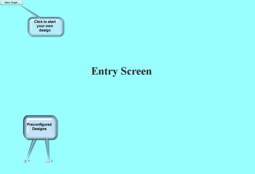
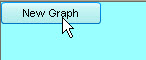
When you start the demonstration you will see a blank screen with a "New Graph" button in the upper left corner of the window and option buttons in the lower left corner of the window. The option buttons are used to show preconfigured applications.
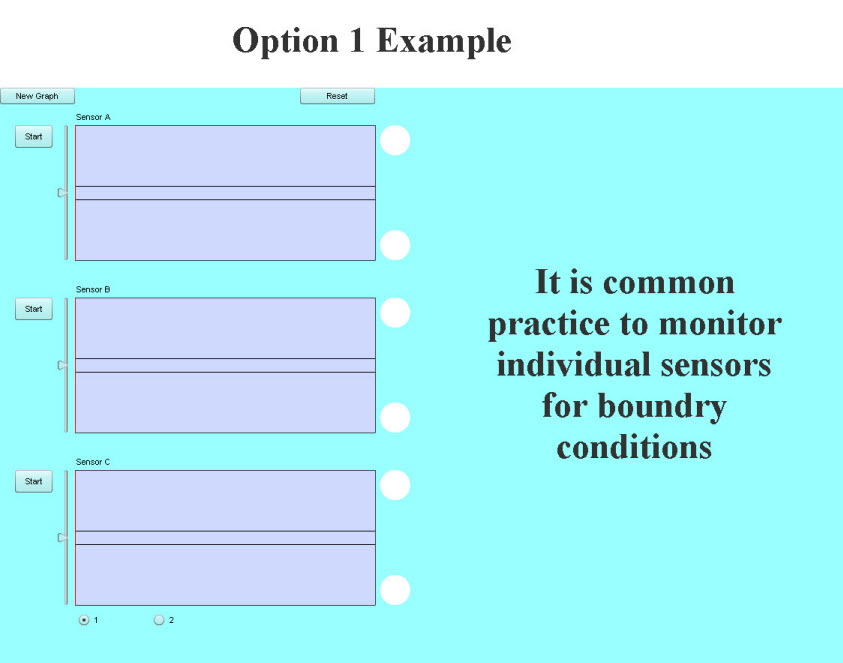
Option 1 shows a conventional unlinked application.
In this case we have three independent sensors, each being monitored for an over and under range alarm.
Click on the Start button to the left of each graph to start monitoring. Adjust the vertical slider to the left of the graph to change the simulated input measurement. The system has been set up to complete a scan in one minute.
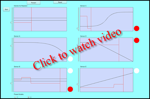
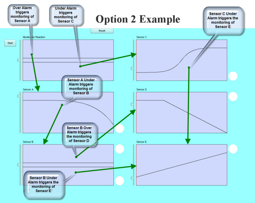
Option 2 shows a more complex model.
In this case we are using Graph 1 (upper left) to monitor for the initial event. When it detects an Over-Range condition, it will start monitoring Sensor A (Graph 2, second down on the left). If it detects an Under-Range condition, it will start monitoring Sensor C (Graph 4, the top right graph). Graph 1 is not being used to trigger alarms (as represented by the lack of alarm indicators to the left of the graph).
Graph 2 (Sensor A) is used to detect an Under-Alarm condition, which is also used to trigger the monitoring of Sensor B (Graph 3, lower left graph).
Graph 3 (Sensor B) is being used to monitor a range. If an abnormally high value is detected, an Over-Alarm condition indicated and it triggers the monitoring of Sensor D (Graph 5). If an abnormally low value is detected, an Under-Alarm condition is indicated and it triggers the monitoring of Sensor E (Graph 6, lower right graph).
Graph 4 (Sensor C - triggered by Graph 1 under range detection) is being monitored for an Under-Alarm condition, which triggers the monitoring of Sensor E (Graph 6). Note that Graph 6 is triggered by either Graph 3 Under-Range, or Graph 4 Under-Alarm. An S curve is used to define the desired alarm conditions.
Graph 5 (Sensor D - triggered by Graph 3 Over-Range) is being monitored for Over-Alarm condition. The limit holds at the upper range for 20 seconds and then declines to 0 at the end of a minute.
Graph 6 (Sensor E - triggered by Sensor B Under-Range and/or Sensor C Under-Alarm) is measured against a straight line for Over-Alarm detection.
To create your own models:
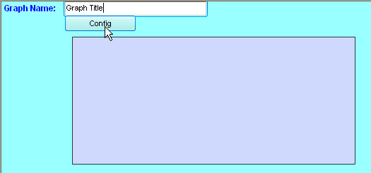
When defining a new graph it is helpful to give it a title. Then click the Config button to select a curve type.
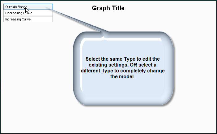
The first step in configuring a curve is to select a type.
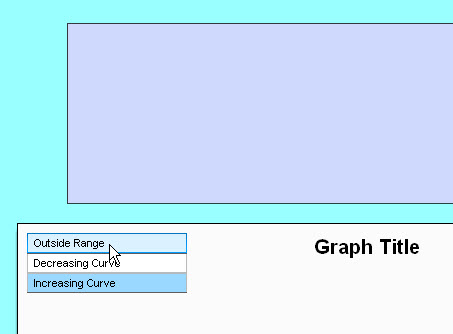
Three types of curves can be used (of course any variety of curves could be generated and packaged in a production application). The "Outside Range" option allows you to pick a value with +/- offset. This would normally be used to monitor a range of selected values for out of range detection. The "Decreasing Curve" supports the situation where you start monitoring a value that you expect will decrease over the scan time (curves down from left to right). The "Increasing Curve" supports the situation where you start monitoring a value that you expect will increase over the scan time (curves from lower left to upper right).
The option that you select will determine what appears in the configuration screen.
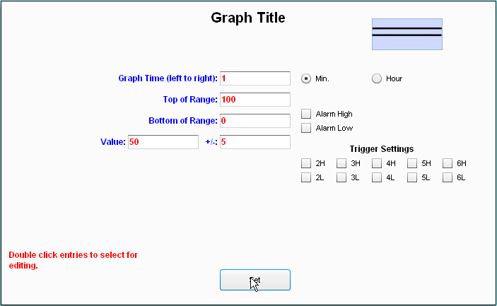
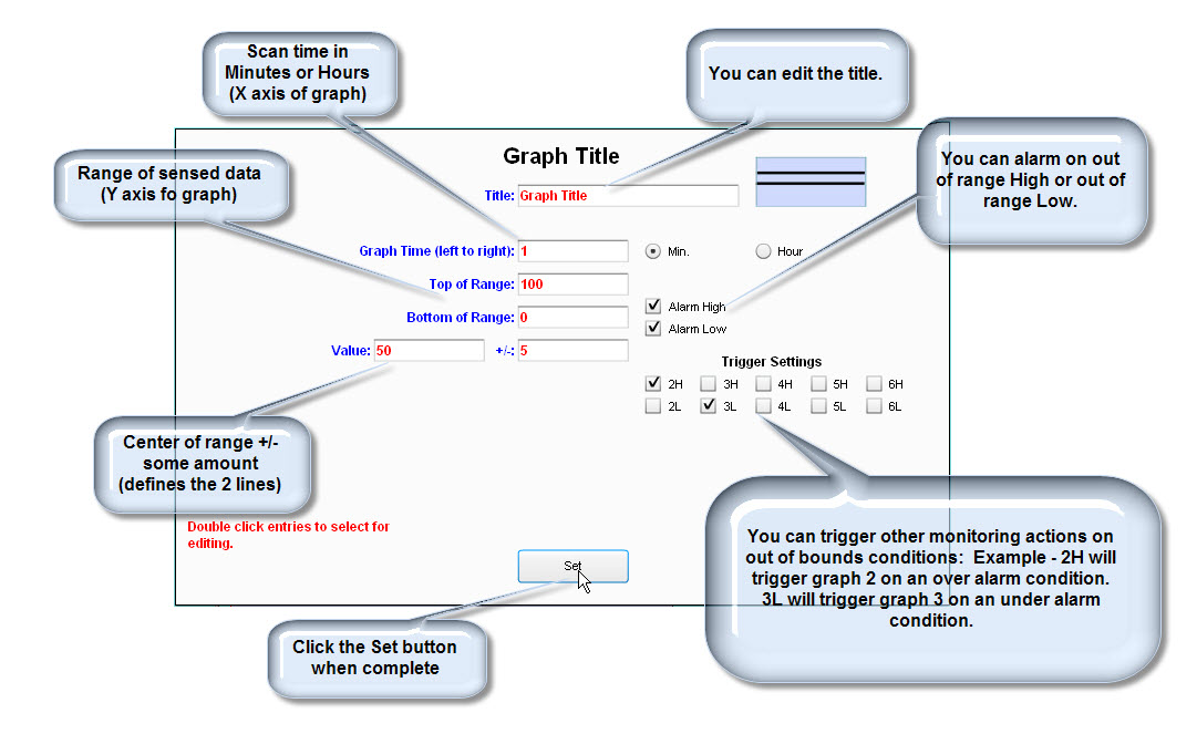
The "Outside Range" configuration screen:
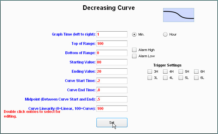
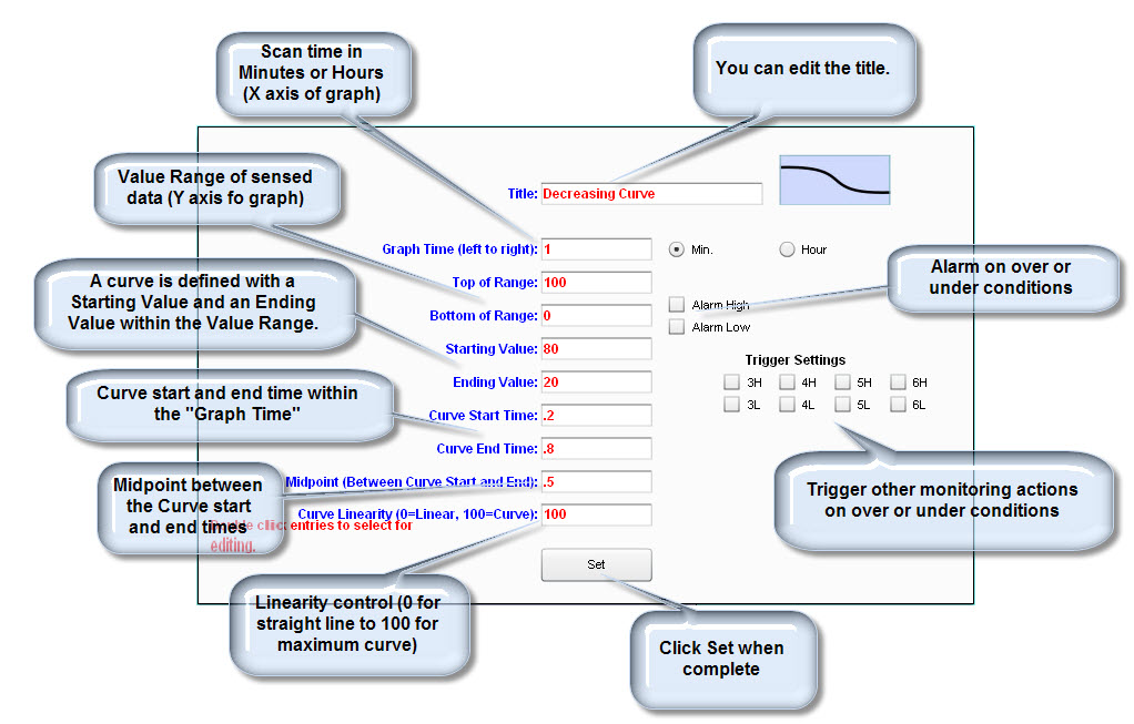
This is the "Decreasing Curve" configuration screen. The "Increasing Curve" configuration screen is similar, with the exception that the Starting Value for a Decreasing Curve must be greater than the Ending Value; and vise versa for the Increasing Curve:
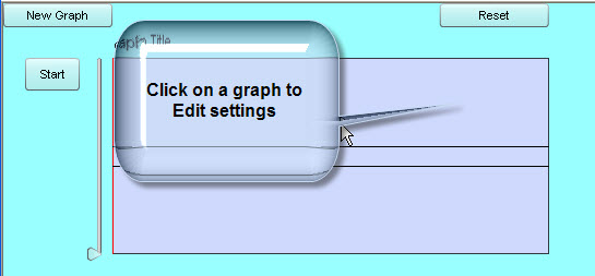
The following screenshot shows three independent graphs created with their default settings. NOTE: When a graph is stand-alone (independent of other factors), a Start Button is displayed to the upper left of each graph. A vertical slider is also provided to the left of each graph to allow the simulation of measured values.
A Reset button is available to remove all the graphs from the screen. Nothing is saved.
Once you have created screens, you may want to edit the configuration values. You can edit an existing design by clicking on the graph on the screen (assuming that you have not started monitoring the sensors).
Editing a Range curve:
Editing an Decreasing Curve or Increasing Curve:
When you click Set, the values for that graph are saved. The graph layout screen is updated with the new values. The curves are redrawn on the screen. The curves are stored as inputs to the embedded KEEL Engines that you tuned using the Configuration screens. When you click "Start", a timer is started that "ticks" every .5 seconds. During each tick the KEEL Engine behind each curve is called with the new sensor data for that graph (from the vertical sliders at the left of each graph).
This present demonstration shows only 2 dimensional graphs, but with KEEL it is easy to have "adaptable curves", or those that could be bent by outside influences.
For example, in the medical case a person's blood pressure may change depending on whether the person is sitting, standing or lying down. If a sensor was integrated with this knowledge, it could be used to shift one or more of the curves up or down and still provide a way to make an intelligent monitoring decision.
|
Copyright , Compsim LLC, All rights reserved |